Plagued by a cryptic clock

Katherine Eaton; Leo Featherstone; Sebastian Duchene; Hendrik Poinar

Plague has an impressively long and expansive history as a human disease. The earliest evidence of the plague bacterium, Yersinia pestis, comes from ancient DNA studies, dating its emergence to at least the Neolithic [1,2]. Since then, Y. pestis has traveled extensively due to ever-expanding global trade networks and the ability to infect a wide variety of mammalian hosts [3,4]. Few regions of the ancient and modern world remain untouched by this disease, as plague has an established presence on every continent except Oceania [5].

Accompanying this prolific global presence is unnervingly high mortality. The infamous medieval Black Death is estimated to have killed more than half of Europe’s population [6]. This virulence can still be observed in the post-antibiotic era, where case fatality rates range from 22-71% [7]. As a result, plague maintains its status as a disease that is of vital importance to current public health initiatives.

This high priority disease status is unsurprising given that Y. pestis is a member of the Enterobacteriaceae family. This family includes other notable pathogens such as Escherichia coli and Salmonella typhi that are commonly transmitted by contaminated food and water. In comparison, the plague bacterium is unique among this family due to a striking difference in host habitat and transmission. Y. pestis commonly resides in the blood of its mammalian hosts and can be transmitted to new hosts through an infectious fleabite [8]. Furthermore, this unique mechanism evolved relatively recently, possibly around the 1st millennium BC [9], long after Y. pestis emerged as a monomorphic clone of the enteric pathogen Yersinia pseudotuberculosis [10].

While the population structure of Y. pseudotuberculosis is well-defined, [11,12], the phylogenetic patterning of Y. pestis remains cryptic. Populations of Y. pestis have been historically categorized according to a a vast array of historical, ecological, biochemical, and molecular characteristics. As a result, disparate sub-typing systems have emerged over the years to differentiate lineages of plague [13]. It has thus been argued that the taxonomy of Y. pestis should be revised and consolidated according to the latest global phylogenetic analysis [14].

Unfortunately, there are a number of obstacles that have stalled large-scale phylogenetic analysis. The first challenge is data availability, both in terms of the genomic sequences, as well as the metadata required for interpretation. Genomic sampling of Y. pestis has recently intensified [15], thus providing exceptional new datasets for statistical inference. This intensive sampling has produced over 1000 Y. pestis genomes that are now publicly available, with tremendous diversity spanning five continents and 5000 years of human history. Unfortunately, the majority of these genomic records lack curated metadata, such as sampling date and location, which are crucial variables in testing population structure.

The second major obstacle is an apparent lack of temporal structure in Y. pestis. Detecting temporal signal and estimating a molecular clock model are general pre-requisites for sophisticated methods of quantifying population structure [16]. However, there has been significant debate concerning whether Y. pestis can be appropriately modeled using the available clock methods [17,18,19]. To some extent, this debate can be explained by different Y. pestis datasets, which have been shown to produce dramatically different patterns of temporal signal [20]. Therefore, it is uncertain whether the new intensively sampled genomes will bring clarity or greater uncertainty.

In response to these debates and obstacles, this paper proposes a theoretical and methodological shift in plague genomics. Rather than conceptualizing Y. pestis as a conglomerate species, we highlight how novel insight emerges through analyzing Y. pestis sub-populations in isolation. To accomplish this shift in discourse, we focus on four objectives, specifically to:

Progress towards these key objectives is anticipated to benefit both prospective studies of plague, such as environmental surveillance and outbreak monitoring, and retrospective studies, which seek to date emergence and spread of past pandemics.

Methods

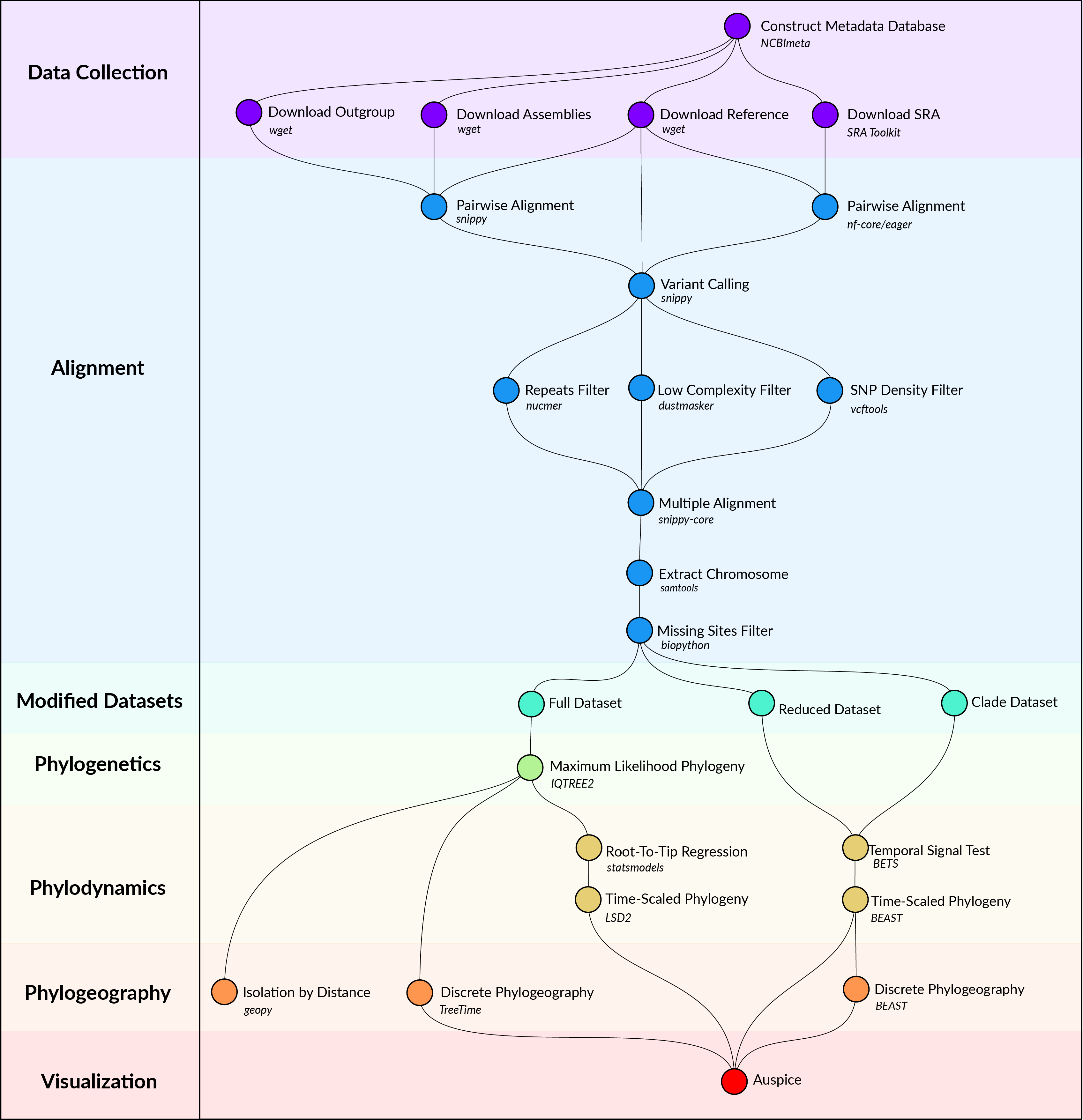
A visual overview of the computational methods is provided in Figure 1 and is available as a snakemake pipeline (https://github.com/ktmeaton/plague-phylogeography/).

Data Collection

Y. pestis genome sequencing projects were retrieved from the NCBI databases using NCBImeta [21]. 1657 projects were identified and comprised three genomic types:

The 887 modern unassembled genomes were excluded from this project, as the wide variety of laboratory methods and sequencing strategies precluded a standardized workflow. In contrast, the 184 ancient unassembled genomes were retained given the relatively standardized, albeit specialized, laboratory procedures required to process ancient tissues. Future work will investigate computationally efficient methods for integrating more diverse datasets.

Collection location, collection date, and collection host metadata were curated by cross-referencing the original publications. Collection location was transformed to latitude and longitude coordinates using GeoPy [22] and the Nominatim API [23] for OpenStreetMap [24]. Coordinates were standardized at a sub-country resolution, taking the centroid of the parent province/state. Collection dates were standardized according to their year, and recording uncertainty arising from missing data and radiocarbon estimates. Collection host was the most diverse field with regards to precision, ranging from colloquial nomenclature (“rat”) to a genus species taxonomy (“Meriones libycus”). For the purposes of this study, collection host was recorded as Human, Non-Human, or Not Available, given the inability to differentiate non-human mammalian hosts.

Genomes were removed if no associated date or location information could be identified in the literature, or if there was documented evidence of laboratory manipulation.

Two additional datasets were required for downstream analyses. First, Y. pestis strain CO92 (GCA_000009065.1) was used as the reference genome for sequence alignment and annotation. Second, Yersinia pseudotuberculosis strains NCTC10275 (GCA_900637475.1) and IP32953 (GCA_000834295.1) served as an outgroup to root the maximum likelihood phylogeny.

Alignment

Modern assembled genomes were aligned to the reference genome using Snippy, a pipeline for core genome alignments [25]. Modern genomes were removed if the number of sites covered at a minimum depth of 10X was less than 70% of the reference genome.

Ancient unassembled genomes were downloaded from the SRA database in FASTQ format using the SRA Toolkit [26]. Pre-processing and alignment to the reference genome was performed using the nf-core/eager pipeline, a reproducible workflow for ancient genome reconstruction [27]. Ancient genomes were removed if the number of sites covered at a minimum depth of 3X was less than 70% of the reference genome. It is a typical approach to relax coverage thresholds for ancient genomes relative to their modern counterparts [cite?]. The threshold chosen here is commonly used, and aims to strike a balance between variant confidence and sample representation [cite?].

A multiple sequence alignment was constructed using the Snippy Core module of the Snippy pipeline [25]. The output alignment was filtered to only include chromosomal variants and to exclude sites that had more than 5% missing data.

Modified Datasets

To investigate the influence of between-clade variation in substitution rates, the multiple alignment was separated into the major clades of Y. pestis, which is referred to as the clade dataset. Clade labeling was derived from the five-branch population structure accompanied by a biovar abbreviation [17]. Only one modification was made, in that the subclade associated with the Plague of Justinian (0.ANT4) was considered to be a distinct clade from its parent (0.ANT) due to its geographic, temporal, and ecological uniqueness.

To improve the performance and convergence of Bayesian analysis, a subsampled dataset was constructed and is referred to as the reduced dataset. Clades that contained multiple samples drawn from the same geographic location and the same time period were reduced to one representative sample. The sample with the shortest terminal branch length was prioritized, to diminish the influence of uniquely derived mutations on the estimated substitution rate. An interval of 25 years was identified as striking an optimal balance, resulting in 191 representative samples.

Phylogenetics

Model selection was performed using Modelfinder which identified the K3Pu+F+I model as the optimal choice based on the Bayesian Information Criterion (BIC) [28]. A maximum-likelihood phylogeny was then estimated across 10 independent runs of IQTREE [29]. Branch support was evaluated using 1000 iterations of the ultrafast bootstrap approximation, with a threshold of 95% required for strong support [30].

Phylodynamics

To explore the degree of temporal signal present in the data, two categories of tests were performed . The first was a root-to-tip (RTT) regression on collection date using the python package statsmodels [31]. Given the relative simplicity of a regression model, the full dataset of 601 genomes was used. For the second test of temporal signal, a Bayesian Evaluation of Temporal Signal (BETS) was conducted. As the complexity of Bayesian modeling is computationally intensive, the reduced dataset (N=191) was used.

Public Resource

The maximum likelihood and Bayesian phylogenetic trees were uploaded to the Nextstrain visualization platform at https://nextstrain.org/community/ktmeaton/plague-phylogeography-projects@main. All curated metadata is available for download via Nextstrain, Github, and Zenodo.

Results and Discussion

Phylogeny

A maximum-likelihood phylogeny was estimated from 603 genomes (600 Y. pestis isolates, 1 Y. pestis reference, and 2 Y. pseudotuberculosis outgroup taxa). Following removal of the outgroup taxa, the alignment was composed of 10,249 variant positions with 3,844 sites shared by at least two genomes. In Figure 2, the maximum-likeilhood phylogeny is visualized alongside the four major taxonomic systems currently used to define the population structure of Y. pestis. These include the major phylogenetic branches, biovars, subspecies, and historical time periods/pandemics.

Population Structure

A comparison of sub-typing systems reveals great uncertainty with regards to Y. pestis population structure. The global phylogeny of Y. pestis can be divided into major branches according to the relative position of the “big bang” polytomy [17]. All lineages that diverged prior to this multifurcation are grouped into Branch 0 and those emerging after are the monophyletic clades Branches 1-4. Because the “big bang” polytomy plays such a central role in this system, there is growing interest in estimating its timing and geographic origins [32]. However, an inability to identify phenotypes distinguishing these major branches poses a significant challenge, and thus the exact epidemiological significance of the “big bang” polytomy remains unclear.

An example of this challenge can be seen in the population structure defined by the biovar system. Y. pestis can be categorized using a suite of metabolic properties into the classical biovars: antiqua (ANT), medievalis (MED), orientalis (ORI), and microtus/pestoides (PE) [33,34,35]. While these divisions don’t fully contradict the major branches, they do considerably shift the defining boundaries between Y. pestis populations.

To further complicate matters, researchers from the Commonwealth of Independent State (CIS) have observed biovar inconsistencies in plague foci surveillance [14]. In response, the subspecies taxonomy was created to distinguish a main subspecies (pestis) that is highly virulent in humans with wide geographic spread, from five or more non-main subspecies that have limited geographic ranges and attenuated virulence in humans [14]. The subspecies structure is highly convenient for laboratory diagnostics in the CIS, but struggles to differentiate the immense diversity represented by the larger pestis subspecies.

The challenge of categorizing plague by metabolism is, unsurprisingly, also an obstacle when analyzing extinct lineages. Ancient DNA (aDNA) researchers have opted to either extrapolate an existing biovar designation [18] or create a new one [9]. However, it is more common in aDNA studies to define population structure by time period and associations with historically documented pandemics. The known genetic diversity of Y. pestis thus far has been broadly grouped into four time periods and three pandemics (Figure 3).

The First Pandemic (6th - 8th century CE) began with the Plague of Justinian and proceeded to devastate the Byzantine Empire of the Mediterranean world [cite?]. The Late Antiquity clade found within Branch 0 (0.ANT4) is associated with this pandemic given spatiotemporal overlap of the skeletal remains from which this lineage was retrieved [18,36]. Similarly, the medieval clade 1.PRE from Branch 1 is thought to derive from the Second Pandemic of Plague. This well-documented pandemic began with the infamous Black Death and swept across most of Eurasia from the 14th to 19th centuries [cite?]. The third documented pandemic of plague, alias the Modern Pandemic, spread globally from the end of the 18th Century and until the mid-20th Century. There is little dispute that a new lineage of plague emerging from Branch 1 as biovar orientalis (1.ORI) was the causative agent of this pandemic. While the World Health Organization (WHO) declared the third pandemic over in 1950 [cite?], this lineage continues to re-emerge to cause localized epidemics such as the 2010 plague in Peru [cite?] and the Madagascar Outbreaks of 2017 [cite?].

While the pandemic clade nomenclature provides an excellent foundation for historical discussion, there are several emergent problems with this system. First is the growing awareness of the spatiotemporal overlap of the Second and the Third Pandemic [cite?]. Previously, the temporal extents of these events were mutually exclusive, dating from the 14th-18th century, and the 19th-20th century respectively. Recent historical scholarship has contested this claim, and demonstrated that these constraints are a product of a Eurocentric view of plague [cite?]. The Second Pandemic is now known to have extended into the 19th Century in parts of the Ottoman Empire, with the latest epidemics dating to 1819 [cite?]. Similarly, the Third Pandemic is now hypothesized to have began as early as 1772 in southern China [37]. It remains unclear where to draw the distinction, if it even exists, between the Second and Third Pandemic.

Another limitation of the pandemic nomenclature is the complete disconnection of Branch 2 to any historical pandemics. This is surprising given that several criteria of a pandemic pathogen are fulfilled by Branch 2 lineages, namely extensive spread and virulence. Branch 2 genomes of Y. pestis have been collected from all throughout Eurasia, stretching from at least the Caucasus, to India, and to eastern China (Figure 4). Furthermore, lineages of Branch 2 have been associated with high mortality epidemics [38] and were observed to have the highest spread velocity of any Y. pestis clade [37] As historical plague scholarship extends beyond the bounds of Western Europe, it will be important to consider the role these lineages played, and adjust nomenclature accordingly.

However, a significant obstacle to understanding the global spread and virulence of past plagues lies in Y. pestis’s weak host associations and a lack of geographic structure. Similar to its parent species, Y. pseudotuberculosis [11], Y. pestis is capable of infecting a wide variety of mammalian hosts [cite?]. But while isolates of Y. pseudotuberculosis cluster by host group [39], the host structure of Y. pestis is cryptic (Figure 5). Most clades are isolated from both humans and non-human animals, although the ancient lineages 0.PRE, (Bronze Age), 0.ANT4 (Late Antiquty) and 1.PRE (Medieval/Early Modern) are exclusively associated with humans. However, this particular exception is largely due to sampling biases, as paleogenomic investigations have historically prioritized human skeletal remains over faunal remains [cite?].

In addition to a cryptic host structure, the geographic patterning of Y. pestis, or lack thereof, reflects a complex dispersal history (Figure 6). Many regions have been colonized by diverse strains of Y. pestis. This diversity can be contemporaneous, such as endemic foci in the Caucausus and Western China (0.PE). Alternatively, this diversity may accrue over multiple centuries through distinct re-introductions and extinctions, as seen through historical clades in Europe (0.ANT, 1.PRE). In these examples, a relatively large amount of genetic diversity appears in a small geographic range (Figure 7). In contrast, regions such as the Americas have been colonized by a single strain of Y. pestis (1.ORI) which shows a relatively small amount of genetic diversity over a tremendously large geographic range.

This geographic complexity is unsurprising given that Y. pseudotuberculosis, the parent species of plague, also does not exhibit strong geographic structure. Outbreak strains of Y. pseudotuberculosis are particularly challenging to cluster, with non-outbreak lineages showing only slightly more geographic signal [39]. In this line of reasoning, the patterning observed in Figure 6 and 7 likely reflects the complex ecology of plague which cycles between endemic reservoirs and epidemic periods.

However, it would be amiss to not acknowledge one of the largest caveats in genomic analyses, which is the issue of sampling bias. The geographic sampling strategy of Y. pestis genomes (Figure 6) does not reflect the known distribution of modern plague [40]. The over-sampling of East Asia has been previously described by [41] and considerably drives the hypothesis that Y. pestis originated in China [17,42]. This once established hypothesis is now in contention, as the most basal strains of Y. pestis (Clades 0.PRE and 0.PE) have been isolated from all across Eurasia.

The sampling strategy of ancient DNA also does not reflect the hypothesized distribution of ancient plague. Historical genomes of Y. pestis have primarily been collected from European archaeological sites, with the most heavily sampled region being Western Europe (See Figure [map_all_branch_major?], 1.PRE).

Phylodynamics

Detecting Temporal Signal

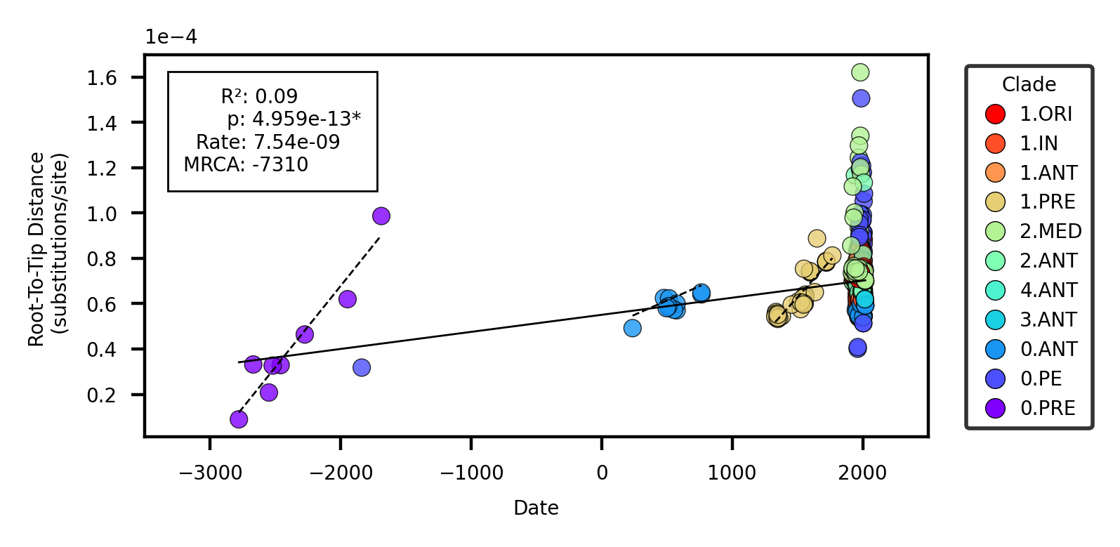
Previous work has documented substantial rate variation both between and within clades of Y. pestis [17,19]. A root-to-tip regression on sampling date for the full dataset (N=601) reproduces this finding as the coefficient of determination (R²) is extremely low at 0.09 (Figure 8). A Bayesian Evaluation of Temporal Signal (BETS) also indicates poor support for a strict clock as the coefficient of variation was consistently estimated to be greater than 1. Taken together, the root-to-tip regression and BETS analysis suggest that alternative clock models, such as the uncorrelated relaxed log normal (UCLN) model, should be preferred when accounting for the high degree of rate variation.

However, the BETS analysis exhibited poor sampling of the relaxed clock model parameters, even when using a fixed topology (Figure 9). This suggests there may be too much rate variation to confidently estimate key parameters such as the mean substitution rate and the time to the most recent common ancestor (tMRCA). This observation is consistent with previous analyses [18] where robust estimates of model parameters could not be estimated, thus leading to the conclusion that Y. pestis lacks temporal signal. At the same time, other studies have suggested data composition is a strong determinant of temporal signal [20] and thus we investigated alternative approaches.

To identify patterns in rate variation that may improve the clock model, we first performed visual inspection of the root-to-tip regression residuals (Figure 8). 3/12 clades appeared to have temporal signal according to a linear model, namely the ancient clades isolated from human skeletal remains: 0.PRE (Bronze Age), 0.ANT4 (Late Antiquity), and 1.PRE (Medieval/Early Modern). Indeed, when the root-to-tip regression was performed on clades in isolation, these three clades demonstrated strong evidence of strict-clock behavior (Table 3, Figure 13). A BETS analysis by clade proved even more sensitive as temporal signal was detected in 7/12 clades (Table 1). Furthermore, for all clades with temporal signal, the relaxed clock model (UCLN) had higher support than the strict clock.

The ubiquitous support for a relaxed clock model was initially surprising, as the root-to-tip regression suggested strict clock-like behavior in several clades. However, this disparity can largely be explained by the known statistical limitations of a root-to-tip regression [43] which assumes either 1) no temporal structure, or 2) temporal structure following a linear model. Thus, a root-to-tip regression is strictly a test of the linear model, and will give no indication that other models are a better fit to the data, ie. a relaxed lognormal model. From this finding, we conclude that a root-to-tip regression is a poor statistical test of temporal signal in Y. pestis, and great caution should be taken in interpreting the associated statistics.

Rate Variation

Our approach of fitting nuanced models segregated by clade reveals that the ‘true’ substitution rates of Y. pestis may be much higher than previously thought. Previous work estimated that Y. pestis has one of the slowest observed substitution rates, around 1-2 x 10^-8, which is on par with the exceptionally slow-evolving Mycobacterium leprae [19]. The BETS analysis on the non-segregated data, which was highly unstable, fell within this published range with a 95% HPD between 1.16 x 10^-8 and 1.95 x 10^-8. However, this global rate is a considerable underestimate, as clades with detectable temporal signal ranged from 2.33 x 10^-8 to 7.70 x 10^-7 (Table 2, Figure 10).

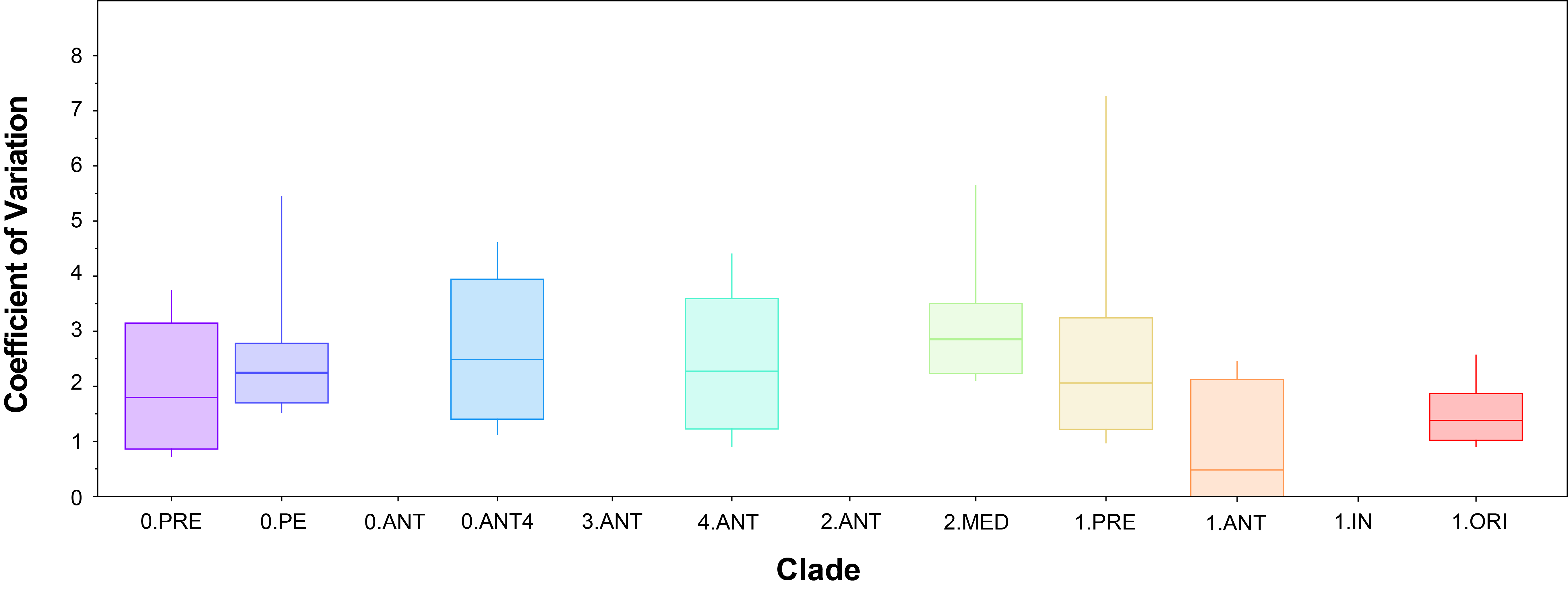
It is interesting to note that several clades have distinctly different substitution rates (ie.non-overlapping estimates of the mean substitution rate in Figure 10) and yet the relative amount of rate variation within a clade is similar (ie. overlapping coefficients of variation in Figure 11).

We hypothesize that outlier clades which are challenging to model (ex. 2.MED) have artificially decreased estimates of the mean substitution rate in past studies. This study therefore reports the substitution rate of Y. pestis to be much higher than previously thought and more comparable to bacteria such as Mycobacterium tuberulcosis.

Node Dating

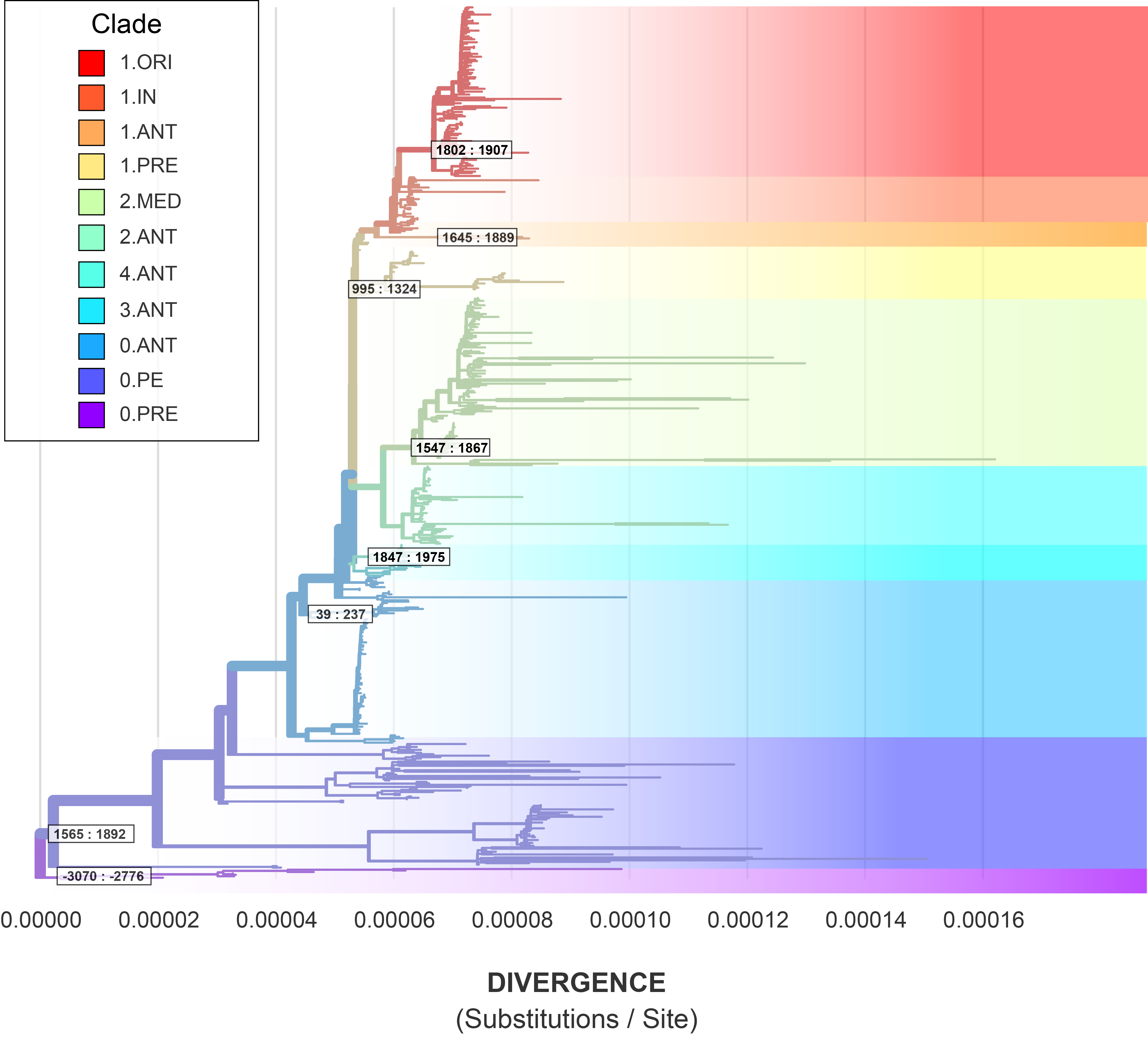
To evaluate the dates associated with ancestral events, we annotated the maximum likelihood phylogeny with the estimated tMRCAs for clades with temporal signal (Figure 12). When re-contextualized into the global phylogeny, the node dates are topologically non-conflicting, meaning that parent nodes correctly pre-date child nodes. The sole exception is the estimated divergence of modern 0.PE which conflicts with the dates associated with the First and Second Pandemic clades. This conflict can be explained by several observations:

This drastic improvement in model performance reveals four intriguing aspects about the evolution of Y. pestis.

The first aspect is that fitting a single clock model to the global phylogeny of Y. pestis is not statistically supported. This can be observed in the relative instability of the MCMC analyses on the reduced dataset, which fails to converge in parameter space. In contrast, successfully fitting models on a clade-by-clade basis reveals that Y. pestis has more temporal signal than previously thought. The observation that different populations have evolved at drastically different rates may explain the previous finding that the apparent structure in Y. pestis is dependent on dataset composition [20].

The final finding from constructing nuanced models concerns the outlier clades for which no detectable signal could be found, namely 0.ANT, 2.ANT, 3.ANT, 2.MED, and 1.IN. The reason for this lack of signal is unclear, but one explanation may be that these Y. pestis populations are inappropriately separated based on the major branch and biovar systems. We hypothesis that alternative strategies to subdivide these populations will yield greater insight, based on the methodological improvements demonstrated in this study.

Conclusion

References

The Stone Age Plague and Its Persistence in Eurasia

Aida Andrades Valtueña, Alissa Mittnik, Felix M Key, Wolfgang Haak, Raili Allmäe, Andrej Belinskij, Mantas Daubaras, Michal Feldman, Rimantas Jankauskas, Ivor Janković, … Johannes Krause

Current Biology (2017-12-04)

DOI: 10.1016/j.cub.2017.10.025 · PMID: 29174893

Emergence and spread of basal lineages of Yersinia pestis during the Neolithic Decline

Nicolás Rascovan, Karl-Göran Sjögren, Kristian Kristiansen, Rasmus Nielsen, Eske Willerslev, Christelle Desnues, Simon Rasmussen

Cell (2019-01-10) https://www.cell.com/cell/abstract/S0092-8674(18)31464-8

DOI: 10.1016/j.cell.2018.11.005 · PMID: 30528431

Trade routes and plague transmission in pre-industrial Europe

Ricci PH Yue, Harry F Lee, Connor YH Wu

Scientific Reports (2017-10-11) https://www.ncbi.nlm.nih.gov/pmc/articles/PMC5636801/

DOI: 10.1038/s41598-017-13481-2 · PMID: 29021541 · PMCID: PMC5636801

Yersinia pestis--etiologic agent of plague

RD Perry, JD Fetherston

Clinical Microbiology Reviews (1997-01)

PMID: 8993858 · PMCID: PMC172914

Plague

World Health Organization

(2017-10-31) https://www.who.int/news-room/fact-sheets/detail/plague

The Black Death, 1346-1353: The Complete History

OJ Benedictow

Boydell Press (2004)

ISBN: 0-85115-943-5

Plague around the world in 2019

Eric Bertherat

Weekly Epidemiological Record (2019-06-21) https://apps.who.int/iris/bitstream/handle/10665/325481/WER9425-en-fr.pdf

Recent trends in plague ecology

K Gage, M Kosoy

(2006) http://reviverestore.org/wp-content/uploads/2015/02/Gage-and-Kosoy_USGS-Blk-footed-ferret-symp_2006-copy.pdf

Early Divergent Strains of Yersinia pestis in Eurasia 5,000 Years Ago

Simon Rasmussen, Morten Erik Allentoft, Kasper Nielsen, Ludovic Orlando, Martin Sikora, Karl-Göran Sjögren, Anders Gorm Pedersen, Mikkel Schubert, Alex Van Dam, Christian Moliin Outzen Kapel, … Eske Willerslev

Cell (2015-10-22) https://www.ncbi.nlm.nih.gov/pmc/articles/PMC4644222/

DOI: 10.1016/j.cell.2015.10.009 · PMID: 26496604 · PMCID: PMC4644222

10.

Yersinia pestis, the cause of plague, is a recently emerged clone of Yersinia pseudotuberculosis

M Achtman, K Zurth, G Morelli, G Torrea, A Guiyoule, E Carniel

Proceedings of the National Academy of Sciences of the United States of America (1999-11-23)

DOI: 10.1073/pnas.96.24.14043 · PMID: 10570195 · PMCID: PMC24187

11.

Population structure of the Yersinia pseudotuberculosis complex according to multilocus sequence typing

Riikka Laukkanen-Ninios, Xavier Didelot, Keith A Jolley, Giovanna Morelli, Vartul Sangal, Paula Kristo, Priscilla FM Imori, Hiroshi Fukushima, Anja Siitonen, Galina Tseneva, … Mark Achtman

Environmental microbiology (2011-12) https://www.ncbi.nlm.nih.gov/pmc/articles/PMC3988354/

DOI: 10.1111/j.1462-2920.2011.02588.x · PMID: 21951486 · PMCID: PMC3988354

12.

Phylogeographic separation and formation of sexually discrete lineages in a global population of Yersinia pseudotuberculosis

Tristan Seecharran, Laura Kalin-Manttari, Katja Koskela, Simo Nikkari, Benjamin Dickins, Jukka Corander, Mikael Skurnik, AlanYR 2017 McNally

Microbial Genomics (2017) https://www.microbiologyresearch.org/content/journal/mgen/10.1099/mgen.0.000133

DOI: 10.1099/mgen.0.000133

13.

Taxonomy of Yersinia pestis

Zhizhen Qi, Yujun Cui, Qingwen Zhang, Ruifu Yang

Yersinia pestis: Retrospective and Perspective (2016) https://doi.org/10.1007/978-94-024-0890-4_3

DOI: 10.1007/978-94-024-0890-4_3 · ISBN: 978-94-024-0890-4

14.

Phylogeny and classification of Yersinia pestis through the lens of strains From the plague foci of Commonwealth of Independent States

Vladimir V Kutyrev, Galina A Eroshenko, Vladimir L Motin, Nikita Y Nosov, Jaroslav M Krasnov, Lyubov M Kukleva, Konstantin A Nikiforov, Zhanna V Al’khova, Eugene G Oglodin, Natalia P Guseva

Frontiers in Microbiology (2018-05-25) https://www.frontiersin.org/article/10.3389/fmicb.2018.01106/full

DOI: 10.3389/fmicb.2018.01106

15.

The EnteroBase user's guide, with case studies on Salmonella transmissions, Yersinia pestis phylogeny, and Escherichia core genomic diversity

Zhemin Zhou, Nabil-Fareed Alikhan, Khaled Mohamed, Yulei Fan, Mark Achtman

Genome Research (2020-01) https://www.ncbi.nlm.nih.gov/pmc/articles/PMC6961584/

DOI: 10.1101/gr.251678.119 · PMID: 31809257 · PMCID: PMC6961584

16.

Identification of Hidden Population Structure in Time-Scaled Phylogenies

Erik M Volz, Wiuf Carsten, Yonatan H Grad, Simon DW Frost, Ann M Dennis, Xavier Didelot

Systematic Biology (2020-09-01) https://doi.org/10.1093/sysbio/syaa009

DOI: 10.1093/sysbio/syaa009

17.

Historical variations in mutation rate in an epidemic pathogen, Yersinia pestis

Y Cui, C Yu, Y Yan, D Li, Y Li, T Jombart, LA Weinert, Z Wang, Z Guo, L Xu, … R Yang

Proceedings of the National Academy of Sciences (2013-01-08) http://www.pnas.org/cgi/doi/10.1073/pnas.1205750110

DOI: 10.1073/pnas.1205750110

18.

Yersinia pestis and the Plague of Justinian 541–543 AD: a genomic analysis

David M Wagner, Jennifer Klunk, Michaela Harbeck, Alison Devault, Nicholas Waglechner, Jason W Sahl, Jacob Enk, Dawn N Birdsell, Melanie Kuch, Candice Lumibao, … Hendrik Poinar

The Lancet Infectious Diseases (2014-04) https://linkinghub.elsevier.com/retrieve/pii/S1473309913703232

DOI: 10.1016/s1473-3099(13)70323-2

19.

Phylogeography of the second plague pandemic revealed through analysis of historical Yersinia pestis genomes

Maria A Spyrou, Marcel Keller, Rezeda I Tukhbatova, Christiana L Scheib, Elizabeth A Nelson, Aida Andrades Valtueña, Gunnar U Neumann, Don Walker, Amelie Alterauge, Niamh Carty, … Johannes Krause

Nature Communications (2019-10-02) https://www.nature.com/articles/s41467-019-12154-0

DOI: 10.1038/s41467-019-12154-0

20.

Genome-scale rates of evolutionary change in bacteria

Sebastian Duchêne, Kathryn E Holt, François-Xavier Weill, Simon Le Hello, Jane Hawkey, David J Edwards, Mathieu Fourment, Edward C Holmes

Microbial Genomics (2016-11-30) https://www.ncbi.nlm.nih.gov/pmc/articles/PMC5320706/

DOI: 10.1099/mgen.0.000094 · PMID: 28348834 · PMCID: PMC5320706

21.

NCBImeta: efficient and comprehensive metadata retrieval from NCBI databases

Katherine Eaton

Journal of Open Source Software (2020) https://doi.org/10.21105/joss.01990

DOI: 10.21105/joss.01990

22.

GeoPy: A Python client for several popular geocoding web services.

Kostya Esmukov

(2020-12) https://github.com/geopy/geopy

23.

Nominatim: A tool to search OpenStreetMap data.

Sarah Hoffman

(2020-12) https://github.com/osm-search/Nominatim

24.

Planet dump retrieved from https://planet.osm.org

OpenStreetMap Contributors

(2017) https://www.openstreetmap.org

25.

Snippy: Rapid haploid variant calling and core genome alignment.

Torsten Seemann

(2020-03-08) https://github.com/tseemann/snippy

26.

ncbi/sra-tools

NCBI - National Center for Biotechnology Information/NLM/NIH

(2021-05-18) https://github.com/ncbi/sra-tools

27.

Reproducible, portable, and efficient ancient genome reconstruction with nf-core/eager

James AFellows Yates, Thiseas C Lamnidis, Maxime Borry, Aida Andrades Valtueña, Zandra Fagernäs, Stephen Clayton, Maxime U Garcia, Judith Neukamm, Alexander Peltzer

PeerJ (2021-03-16) https://peerj.com/articles/10947

DOI: 10.7717/peerj.10947

28.

ModelFinder: fast model selection for accurate phylogenetic estimates

Subha Kalyaanamoorthy, Bui Quang Minh, Thomas KF Wong, Arndt von Haeseler, Lars S Jermiin

Nature Methods (2017-06) http://www.nature.com/articles/nmeth.4285

DOI: 10.1038/nmeth.4285

29.

IQ-TREE 2: New Models and Efficient Methods for Phylogenetic Inference in the Genomic Era

Bui Quang Minh, Heiko A Schmidt, Olga Chernomor, Dominik Schrempf, Michael D Woodhams, Arndt von Haeseler, Robert Lanfear

Molecular Biology and Evolution (2020-05-01) https://academic.oup.com/mbe/article/37/5/1530/5721363

DOI: 10.1093/molbev/msaa015

30.

UFBoot2: Improving the Ultrafast Bootstrap Approximation

Diep Thi Hoang, Olga Chernomor, Arndt von Haeseler, Bui Quang Minh, Le Sy Vinh

Molecular Biology and Evolution (2018-02-01) https://academic.oup.com/mbe/article/35/2/518/4565479

DOI: 10.1093/molbev/msx281

31.

Statsmodels: Econometric and Statistical Modeling with Python

Skipper Seabold, Josef Perktold

(2010) https://conference.scipy.org/proceedings/scipy2010/seabold.html

DOI: 10.25080/majora-92bf1922-011

32.

How a microbe becomes a pandemic: a new story of the Black Death

Monica H Green

The Lancet Microbe (2020-12-01) https://www.thelancet.com/journals/lanmic/article/PIIS2666-5247(20)30176-2/abstract

DOI: 10.1016/s2666-5247(20)30176-2

33.

Variétés de l'espèce Pasteurella pestis

R Devignat

Bulletin of the World Health Organization (1951) https://www.ncbi.nlm.nih.gov/pmc/articles/PMC2554099/

PMID: 14859080 · PMCID: PMC2554099

34.

Comparative and evolutionary genomics of Yersinia pestis

Dongsheng Zhou, Yanping Han, Yajun Song, Peitang Huang, Ruifu Yang

Microbes and Infection (2004-11-01) http://www.sciencedirect.com/science/article/pii/S1286457904002357

DOI: 10.1016/j.micinf.2004.08.002

35.

Genotyping and Phylogenetic Analysis of Yersinia pestis by MLVA: Insights into the Worldwide Expansion of Central Asia Plague Foci

Yanjun Li, Yujun Cui, Yolande Hauck, Mikhail E Platonov, Erhei Dai, Yajun Song, Zhaobiao Guo, Christine Pourcel, Svetlana V Dentovskaya, Andrey P Anisimov, … Gilles Vergnaud

PLOS ONE (2009-06-22) https://journals.plos.org/plosone/article?id=10.1371/journal.pone.0006000

DOI: 10.1371/journal.pone.0006000

36.

Ancient Yersinia pestis genomes from across Western Europe reveal early diversification during the First Pandemic (541–750)

Marcel Keller, Maria A Spyrou, Christiana L Scheib, Gunnar U Neumann, Andreas Kröpelin, Brigitte Haas-Gebhard, Bernd Päffgen, Jochen Haberstroh, Albert Ribera i Lacomba, Claude Raynaud, … Johannes Krause

Proceedings of the National Academy of Sciences (2019-06-18) https://www.pnas.org/content/116/25/12363

DOI: 10.1073/pnas.1820447116 · PMID: 31164419

37.

Wet climate and transportation routes accelerate spread of human plague

Lei Xu, Leif Chr Stige, Kyrre Linné Kausrud, Tamara Ben Ari, Shuchun Wang, Xiye Fang, Boris V Schmid, Qiyong Liu, Nils Chr Stenseth, Zhibin Zhang

Proceedings of the Royal Society B: Biological Sciences (2014-04-07) https://royalsocietypublishing.org/doi/10.1098/rspb.2013.3159

DOI: 10.1098/rspb.2013.3159

38.

Evolution and circulation of Yersinia pestis in the Northern Caspian and Northern Aral Sea regions in the 20th-21st centuries

Galina A Eroshenko, Nikolay V Popov, Zhanna V Al’khova, Lyubov M Kukleva, Alina N Balykova, Nadezhda S Chervyakova, Ekaterina A Naryshkina, Vladimir V Kutyrev

PLOS ONE (2021-02-11) https://journals.plos.org/plosone/article?id=10.1371/journal.pone.0244615

DOI: 10.1371/journal.pone.0244615

39.

Genomic Insights into a Sustained National Outbreak of Yersinia pseudotuberculosis

Deborah A Williamson, Sarah L Baines, Glen P Carter, Anders Gonçalves da Silva, Xiaoyun Ren, Jill Sherwood, Muriel Dufour, Mark B Schultz, Nigel P French, Torsten Seemann, … Benjamin P Howden

Genome Biology and Evolution (2016-12-01) https://doi.org/10.1093/gbe/evw285

DOI: 10.1093/gbe/evw285

40.

Historical and genomic data reveal the influencing factors on global transmission velocity of plague during the Third Pandemic

Lei Xu, Leif C Stige, Herwig Leirs, Simon Neerinckx, Kenneth L Gage, Ruifu Yang, Qiyong Liu, Barbara Bramanti, Katharine R Dean, Hui Tang, … Zhibin Zhang

Proceedings of the National Academy of Sciences (2019-06-11) https://www.pnas.org/content/116/24/11833

DOI: 10.1073/pnas.1901366116 · PMID: 31138696

41.

Historical Y. pestis Genomes Reveal the European Black Death as the Source of Ancient and Modern Plague Pandemics

Maria A Spyrou, Rezeda I Tukhbatova, Michal Feldman, Joanna Drath, Sacha Kacki, Julia Beltrán de Heredia, Susanne Arnold, Airat G Sitdikov, Dominique Castex, Joachim Wahl, … Johannes Krause

Cell Host & Microbe (2016-06) http://linkinghub.elsevier.com/retrieve/pii/S1931312816302086

DOI: 10.1016/j.chom.2016.05.012

42.

Yersinia pestis genome sequencing identifies patterns of global phylogenetic diversity

Giovanna Morelli, Yajun Song, Camila J Mazzoni, Mark Eppinger, Philippe Roumagnac, David M Wagner, Mirjam Feldkamp, Barica Kusecek, Amy J Vogler, Yanjun Li, … Mark Achtman

Nature Genetics (2010-12)

DOI: 10.1038/ng.705 · PMID: 21037571 · PMCID: PMC2999892

43.

Bayesian Evaluation of Temporal Signal in Measurably Evolving Populations

Sebastian Duchene, Philippe Lemey, Tanja Stadler, Simon YW Ho, David A Duchene, Vijaykrishna Dhanasekaran, Guy Baele

Molecular Biology and Evolution (2020-11-01) https://doi.org/10.1093/molbev/msaa163

DOI: 10.1093/molbev/msaa163

Clade	N	SC Bayes Factor	UCLN Bayes Factor	Clock Model
1.ORI	117	29.6*	35.7*	UCLN
1.IN	39	-3.9	-10.2	UCLN
1.ANT	4	8.9*	12.6*	UCLN
1.PRE	40	10.1*	44.1*	UCLN
2.MED	116	TBD	TBD	TBD
2.ANT	54	-20.8	-13.7	UCLN
4.ANT	11	-2.9	3.7*	UCLN
3.ANT	11	-9.6	-11.4	UCLN
0.ANT	103	-2.3	-6.5	UCLN
0.ANT4	12	5.3*	5.9*	UCLN
0.PE	83	-82.1	12.4*	UCLN
0.PRE	8	TBD	TBD	TBD

Plagued by a cryptic clock

Authors

Abstract

Introduction

Methods

Data Collection

Alignment

Modified Datasets

Phylogenetics

Phylodynamics

Public Resource

Results and Discussion

Phylogeny

Population Structure

Phylodynamics

Detecting Temporal Signal

Rate Variation

Node Dating

Conclusion

References

Appendix

Phylodynamics

Root to Tip Regression

Geography

Clade	N	Substitution Rate	Coefficient of Variation	tMRCA
All	191	1.16 x 10^-8 : 1.95 x 10^-8	1.35 : 2.10	-7400 : -3289
1.ORI	117	1.04 x 10^-7 : 1.53 x 10^-7	1.02 : 1.87	1802 : 1907
1.IN	39	–	–	–
1.ANT	4	3.61 x 10^-8 : 9.63 x 10^-8	0.00 : 2.12	1645 : 1889
1.PRE	40	3.69 x 10^-8 : 5.90 x 10^-8	1.22 : 3.24	995 : 1324
2.MED	116	1.91 x 10^-7, 3.01 x 10^-7	2.23 : 3.50	1547 : 1867
2.ANT	54	–	–	–
4.ANT	11	3.59 x 10^-8 : 1.57 x 10^-7	1.22 : 3.59	1847 : 1975
3.ANT	11	–	–	–
0.ANT	103	–	–	–
0.ANT4	12	2.33 x 10^-8 : 4.68 x 10^-8	1.40 : 3.94	39 : 237
0.PE	83	4.32 x 10^-7 : 7.70 x 10^-7	1.70 : 2.78	1565 : 1892
0.PRE	8	3.95 x 10^-8 : 6.48 x 10^-8	0.84 : 3.13	-3070 : -2776

Clade	N	Coefficient	p
All	601	0.09	4.959e-13*
1.ORI	117	0.04	1.184e-01
1.IN	39	-0.0	1.0
1.ANT	4	0.45	1.0
1.PRE	40	0.76	2.022e-12*
2.MED	116	0.01	1.0
2.ANT	54	0.05	4.764e-01
4.ANT	11	-0.11	1.0
3.ANT	11	-0.04	1.0
0.ANT	103	-0.01	1.0
0.ANT4	12	0.66	7.842e-03*
0.PE	83	0.01	1.0
0.PRE	8	0.91	1.678e-03*